


Variance and Match Length in Tennis
A statistical explanation for the effect of match length on elite performance

A well-recognized fact of tennis is that the best players are more likely to lose in smaller tournaments than larger ones.1 For example, from 2004-2022, the “Big 3” — Federer, Nadal, and Djokovic — won 84% of the Grand Slams (61/72) but just 61% of the ATP 1000 Masters tournaments (100/163).
A common and intuitive explanation for this discrepancy is that better players “pull through” when it counts for more. The idea here is that top players may put forth less effort in smaller tournaments, either because the stakes are lower or because they are saving themselves for larger tournaments. This theory certainly appears to have purchase in such leagues as the NBA, where players like Lebron James and Kobe Bryant are known to improve their quality of play in the playoffs.
While perhaps true, these theories miss a much simpler explanation for the discrepancy in winning percentages. Unlike Grand Slams which are played as best of five sets, smaller ATP events are played as best of three sets — crowning the first player to win 2 sets. This small difference may seem inconsequential, but in stochastic environments, reducing the sample size can significantly increase the variance of match outcomes. Just as a flipping 60% heads on a fair coin is more common on 10 flips than 100 flips, winning a match is a surer bet for a better player over a longer frame of reference.
In the remainder of this post, I derive formally how match length affects winning probability under some simplifying assumptions. Turning to the data, I explore how far this model goes in explaining the discrepancy in tournament performance. The basic result: not very far! Using fitted data, match length explains just 10% of the decreased performance exhibited by top players in Masters tournaments relative to Grand Slams. The remaining 90% is explained by other factors, such as diminished playing ability or compositional changes in opponent quality.
Model
Suppose a tennis player (call him Roger) wins a set against another player (call him Rafael) with probability p. Further assume — contra reality — that sets are independent of one another: that is, the outcome of one set has no bearing on the next. We are interested in how the probability of winning any given set translates into the probability of winning the match as a whole.
Clearly, this probability depends on the length of the match. On a best of three (BO3) set match, there are 3 possible outcomes for Roger in terms of sets won (W) and lost (L): {WW,WLW,LWW}. Given that W occurs with probability p, the probability of {WW} is p^2 and the probability of {WLW} and {LWW} are each p^2(1-p). The probability Roger wins is therefore:

Consider now a best of five (BO5) set match. Using the same logic as before, the probability that Roger wins is the sum of probabilities that Roger wins in three, four, and five sets respectively:

There is a nice general form for this distribution. The probability a player wins a best of n set match (m:=(n+1)/2 is the number of sets that a player must reach to win) is given by:2

There are a couple of things to note about this distribution. First, as n grows without bound, better players — those with p>0.5 — win the match almost surely. Worse players — those with p<0.5 — lose the match almost surely:

Second, the distribution both for n large and n small varies wildly with p. With p=0.65, a player has an 80% chance of winning in a best of 3 set match. With p=0.55, a player does not achieve a 80% probability of winning the match until best of 35 sets!! An immediate consequence of this nonlinearity is that, looking at match outcomes alone, it can take an extremely long time to differentiate players who are marginally different in terms of ability.
The original purpose of this post was to consider how the probability of winning differs in best of 5 set matches (Grand Slams) vs. best of 3 set matches (all other ATP events). To that end, consider the match win probabilities across different player abilities according to our model.
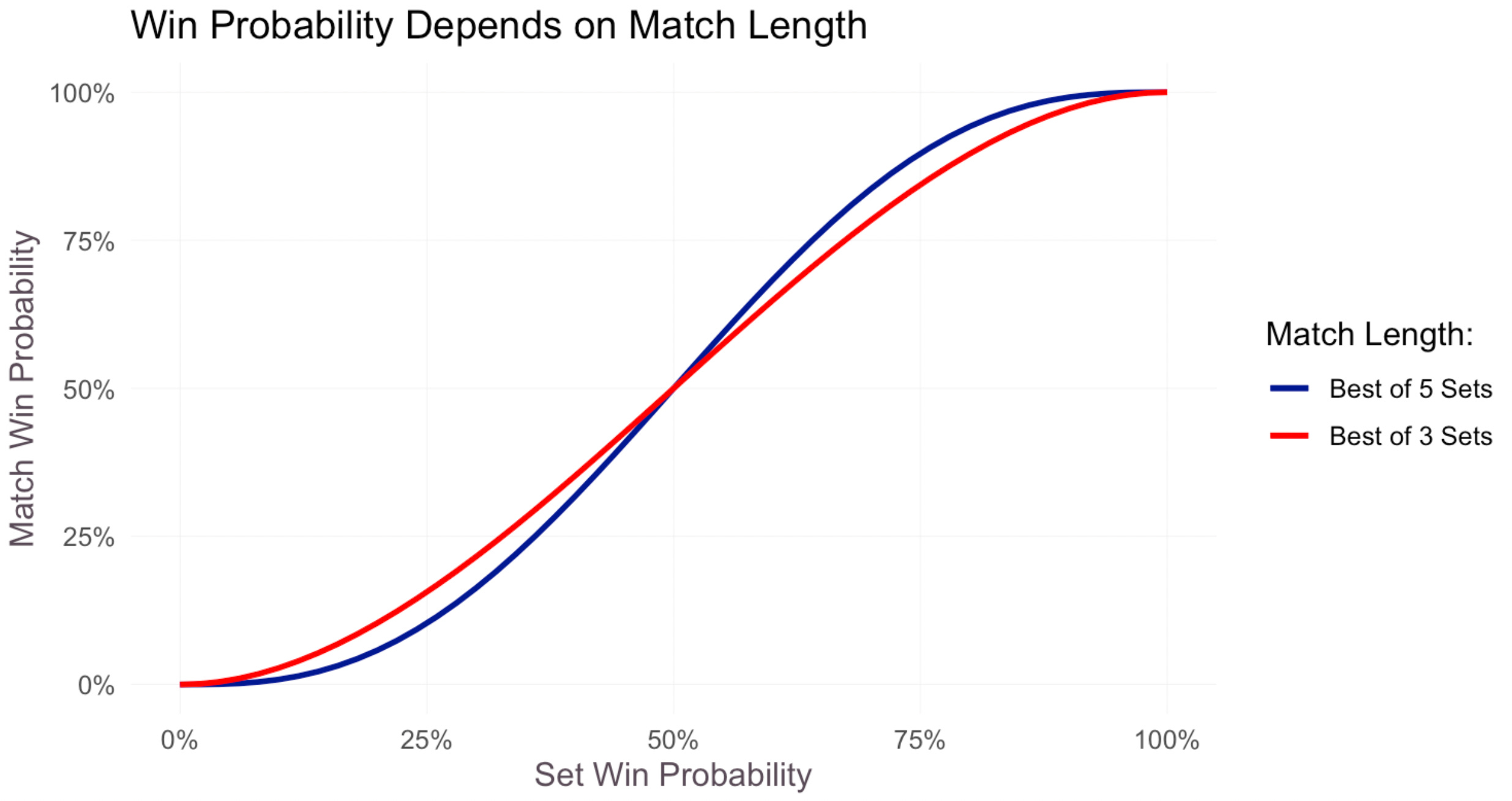
The probability of winning a match is obviously increasing in the probability of winning a set (hence both lines increasing), but varies based on match length. In a BO3 set match (red line), the probabilities of winning a match shrink toward 50%; that is, the match outcome is more noisy. This higher variance aids worse players (red > blue for p<0.5) and harms better players (blue > red for p>0.5).
To capture this differential impairment explicitly, we can plot the red line minus the blue line, which tells us for each level of ability, how large is the reduction in win probability when the player competes in a BO3 match vs. a BO5 match:

Here the difference is more apparent: a player who wins 70% of his sets will, on average, win 5% fewer short matches than long matches. On the other hand, a player who wins 40% of his sets is expected to win 3.5% more short matches than long matches. To be clear, these results are purely a function of the higher variance associated with smaller sample sizes. They only assume that ability — parametrized by probability of winning a set — is the same in short and long matches.
Data
Just how far can we get with this model in the real world? And are its assumptions even reasonable to begin with? Thanks to Jeff Sackmann’s excellent tennis database, we can address these questions ourselves.
I construct the table below to illustrate the answers to both questions. Among top players, and in contrast to our modeling assumption, it is indeed the case that sets are won with higher probability at Grand Slams than at Masters tournaments. Federer, for example, wins 4.9% fewer sets in Masters tournaments than in Grand Slams. This difference could very well be attributable to the higher effort in Grand Slams or perhaps due to the composition of his opponents.

More pertinent to this article, the deterioration in match win percent (the final column) exceeds the deterioration in set win percentages across the board. Federer wins 4.9% fewer sets in shorter tournaments, but 7.0% fewer matches. With the exception of Medvedev, this inequality holds across the board. Stated differently, the shorter match length reduces the win percentages of top players more than is suggested by the change in performance alone.
At the bottom of the distribution, we see similar results.

Here the results are somewhat noisier by nature, but the basic idea still holds. Set performance improves for the worst players in Masters tournaments, but their performance in matches improves even more.
Decomposition
The data above suggest that the difference in outcomes is due to both changes in performance and changes in match length. As a final exercise, we can attempt to measure the relative contributions of these two effects. Suppose we have a model f(p,n) that takes a set win probability p and a match length (best of n) and translates it in a match win probability. We are interested in:

Put simply, this equation states: how much of the change in match win rate is due to differences in set win rate (holding match length fixed) vs. differences in match length (holding set win rate fixed)? Together these effects must sum to the total difference.
Because decomposition requires the estimation of counterfactual outcomes, we require a model for wins as a function of set win rate and match (f(p,n)). We gave one such model in equation (1) above, but to the extent it’s a bad model, our decomposition will be biased. Instead we can fit functions f(p,3) and f(p,5) from the data using logistic regression. Below, we show the fits of different lines against the actual data.
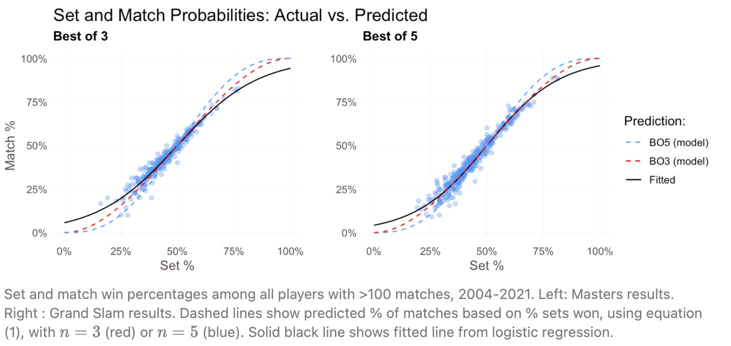
The fitted data predicts a much smaller effect of match length than does our binomial model. Replicating the previous figures using the fitted regression lines, the largest effect of match length is just over 2%, compared to the 5% difference in our original model.

Using these fitted curves, as well as the empirical differences in the performance, we can compute the contribution of match length as:

We plot the density below for the top 40 players in the tour. The mode of the distribution gives our top-line result previously reported. The main takeaway: just 10% of the worse performance of top players in Masters tournaments is due to the shorter match length. The other 90% is due to differences in performance!

It is tempting to conclude that 90% of the difference in outcomes is due to effort. But a much more salient explanation is simply that the quality of opponents differs across the two match types. Below, I plot the distribution of opponent ranks for the top 40 players in Masters vs. Grand Slam tournaments.

Clearly, the distribution of opponents in Masters tournaments peaks earlier (i.e. at higher ranks): the median opponent in a Master’s tournament is ranked approximately 10 spots higher than the median Grand Slam opponent. Differences in opponent quality are obviously first order in explaining performance and will mechanically lower the share of the difference we can attribute to match length. What this implies for our analysis is that, if anything, 10% is a lower bound for the estimate. If we could control for opponent quality, the effect of match length on outcomes would be even larger.
In addition to opponent quality, one final caveat worth mentioning is that match length may operate in more complex ways than scaling variance due to noise. There may be something special about how worse players simply cannot sustain a high quality of play for more than one or two sets. In this case, a longer match would aid the better player both by increasing sample size and by wearing down the opponent. (This is why its better to design series that are multiple games, rather than one very long game!)
Conclusion
The broad takeaway of this piece is that shorter matches reduce the win rate of the best players by as many as 2 percentage points and account for at least a tenth of the so-called “underperformance” of top players in Masters tournaments. Admittedly, these results are based on somewhat back-of-envelope calculations, but speak to an important phenomenon in sports analytics. Much of the reason why Grand Slam matches are longer — or why NBA and MLB finals are designed as multi-game series — is to better identify the superior competitor. This post developed one analytic framework for thinking about these effects.
A number of interesting economic questions naturally follow: (how) are differences in match length priced in Vegas odds? If performance isn’t independent — for example due to momentum effects or mean reversion — how should we think about variance? Finally, how does optimal strategy change (for better or worse players) in response to different match lengths?
Full post: https://benmarrow.notion.site/Variance-and-Match-Length-in-Tennis-febc18d724394f59a4521c33fd6833b7
I am grateful to Isaac Rose-Berman and Ching-Tse Chen for comments.