
Realized Returns, Expected Returns, and Discount Rates
The dynamics of returns in response to interest rate changes

Introduction
In this post, I explain a simple but under-appreciated result about the dynamics of asset returns in response to changes in discount rates. The basic point is that increases in discount rates co-move negatively with current returns and positively with future returns. This implies that one change in the discount rate — a single increase or decrease — will induce a “reversing” or hump-shaped response in realized returns. Not only is this non-intuitive, but it complicates how we can use returns to measure discount rate shocks.
Example
Suppose an asset operates at a steady state where it enjoys a constant expected return of r. That is, each period it achieves a return of, say, 5% that in a rational world reflects compensation for the risk it imposes on an investor’s portfolio. While this example speaks generally in terms of risky assets, the logic here will apply to interest rates on any asset — mortgage rates and house prices, interest rates and treasuries, etc.
Abstracting from idiosyncratic noise, the realized return of this asset (i.e. the actual change in prices) and expected return (i.e. another term for discount rate) are the same — 5% in our example. Since the price series must also grow at this rate, we achieve straightforward shapes for the three series:

Now suppose that one day, investors wake up and unanimously decide that the asset is more risky than they previously thought: they now demand 8%, rather than 5% return to compensate them for this risk. Importantly for this example, investors do not change their view on expected cashflows: that is, they expect the same dividends over time. How do expected returns, prices, and realized returns change?
Before looking at the immediate impact, let’s first consider the long run behavior. In the new steady state long run, the expected returns on the asset, by construction, are 8%: this is the compensation investors demand (and so must receive) to hold the asset. In other words, in the long run, the one-period realized returns will attain the same level as the new expected return, just as we saw in figure 1.
The interesting dynamics occur in the interim transition to this long run. At the time of the increase in discount rate, the price of the asset must drop. Intuitively, the asset is now less attractive since it is riskier, so demand falls. So the immediate response is a drop in price, i.e. negative realized returns. Combining these two effects, a single increase in discount rates causes negative short run returns and positive long run returns.

We can see this illustrated in Fig 2. The first panel, expected returns, restates the thought experiment: investors start out with discount rates of 5% that rise to 8% at t=9. The second panel shows the price response, which features a drop at t=9 when investors find the asset less attractive. Thereafter, returns must grow at the new level of 8% to compensate investors for returns. The rightmost panel of Fig. 2 illustrates the full dynamics of the return response, first turning negative then rising above the previous steady state.
Implications
To many economists, the dynamics described above should be obvious. So why write about it? The first answer is that this result, while straightforward, is perhaps non-intuitive. It’s strange to think that a one-time, uni-directional increase in a constant parameter — in this case increasing an asset’s discount rate — can induce a response that has different effects in the long and short run on the return of that asset. In simple models, we often think of single causes having effects in a single direction. Here, the reason for the observed response is that expected returns and future realized returns move in the same direction; expected returns and current realized returns move in the opposite direction. In fact, it is precisely because prices are low that future returns can compound at a greater rate. This is also the reason for the “non-intuitive” result that higher interest rates lead to lower returns on bond portfolios.
But the main implication I wanted to write about is how these dynamics affect how we should think about measurement. Financial economists frequently develop theories around discount rate shocks — for example, identifying an event that leads to higher discount rates. The challenge to this agenda is showing that the observed data is consistent with the theorized movements. But when returns have a dynamic response, it can be difficult to conduct empirics. Depending on the window of measurement, the observed return response can be negative, positive, or zero.
To see this, suppose we are operating in the world in the example, with an increase in discount rates from 5% to 8% at some time period t=9. If the economist observes period-by-period data, series similar to those in Fig. 2 would support his theory. But suppose instead the economist only observes prices less frequently, say every two periods. In this case, the realized return may smooth over the precise movements in the realized return series and make it more difficult to identify the recognizable shape.
Fig 3. illustrates this thought experiment, by considering an economist who differs in the frequency of prices he observes. In blue, we show the economist who sees prices every periods, and so can trace out the predictable response to a discount rate shock. But as the frequency moves lower, the annualized returns reflect less of the zigzag shape. For the economist who only observes prices every 8 periods — plotted in the dashed navy line — it may be difficult to differentiate the pattern from standard volatility in the asset. At the very extreme, an economist who only views prices once — say at period 1 and period 17, would only ever see a positive annualized return. The lesson here is that “quick” changes in discount rates may be difficult to measure at low frequencies, since the negative short run movements and positive long run movements will cancel out.

A related concern involves the choice of window for analyzing a discount rate shock. Suppose the economist is unsure about the precise period when a discount rate shock occurs, but correctly believes it occurs sometimes around t=9. One way to test his theory — that avoids the issues with measurement frequency — is to split the sample into a conjectured pre-shock and post-shock period, and compare the averages of one-period returns in the two periods. To illustrate on the figure below, we would omit the grey area from the sample, and simply compare the part after the grey area (8% realized returns) to the time prior (5% realized returns). Taking the difference between the average returns in the pre- and post- period would correctly identify a 3% shock to discount rates.

The complication arises if the economist mis-specifies the window — for example, starting it too early or late. Suppose the investor starts the window at t=10 rather than t=9:
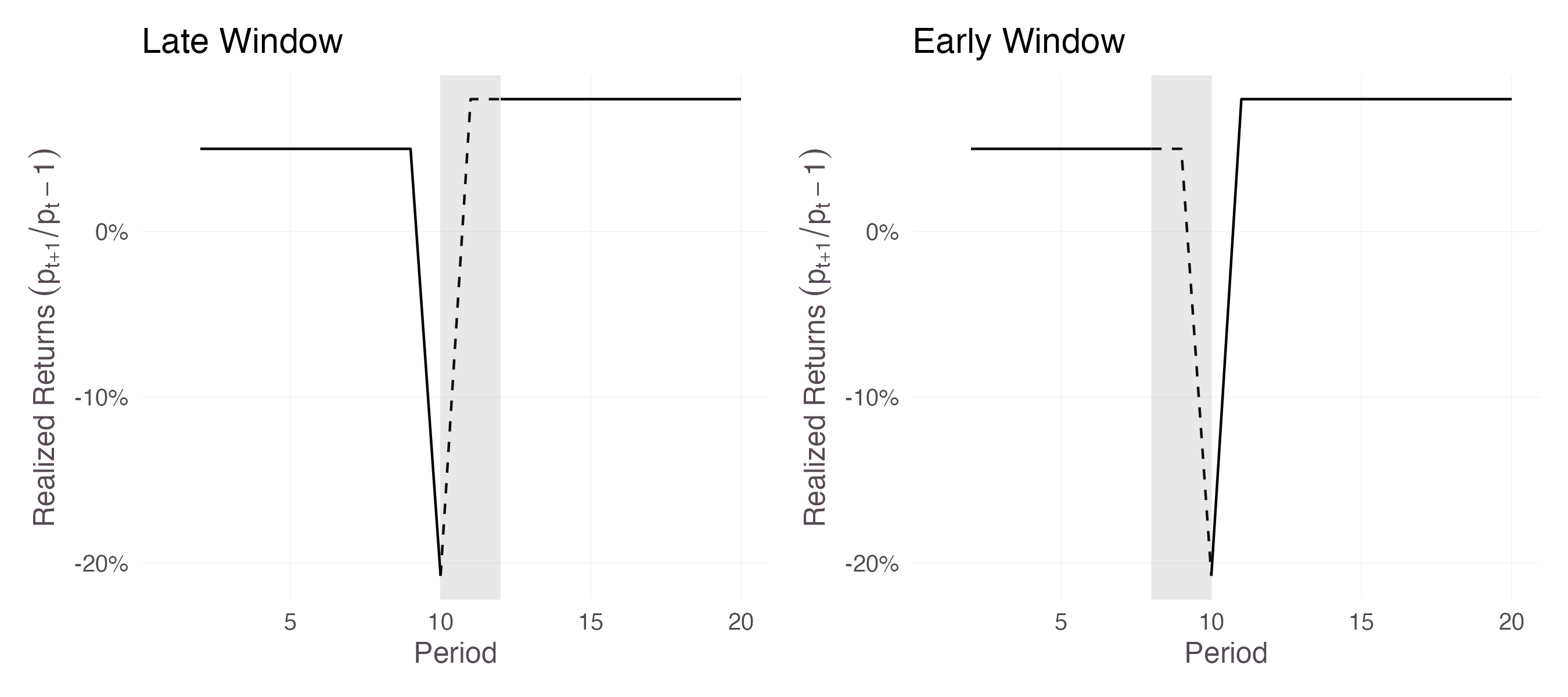
With a late window, as in the left panel of figure 5, the perceived pre-period now includes the shock-induced negative returns. Comparing the post to the pre will then overstate the true difference — the pre-period has artificially low realized returns — and the estimated discount rate shock would be 5.8%. If the window starts too early, as in the right panel of figure 5, the negative return is included in the post-period. Here the estimated effect would shrink to 0.3%. Selecting a correct window may seem like a simple exercise in the single shock, single asset example we analyze here, but more commonly, economists analyze a cross-section of assets with possibly different treatment timing and duration(s), compounded by idiosyncratic movements in the stock price. In these cases, it can be extremely difficult to identify the appropriate window.
Finally, tracing out both directions of the return response can be important if the economist seeks to distinguish a discount rate shock from other types of shock that could determine prices. While a well-identified (i.e. causal) drop in prices is consistent with an increase in the discount rate, it is also consistent with investors lowering their view on the expected payouts of the asset. Distinguishing between these two channels has become an important part of financial research over the past two decades, and the longer term response of realized returns to changes in discount rates provides one way to do it. Although negative returns can be explained by either depressed cash flows or higher discount rates, only the discount rate channel predicts that realized returns will subsequently increase.
Conclusion
The point of this post is to summarize the opposing effects that changes in discount rates have on returns in the short run and long run. This is a simple point, but one that I find to be frequently misunderstood even by well-trained economists. That discount rate shocks affect current and future returns differently is not only theoretically interesting, but also has implications for carrying out empirical work, in everything from estimating effect sizes to distinguishing cash flow from discount rate channels.
I’ll conclude with several other observations that tie in closely with the themes explored above:
Private Equity Returns and Volatility: A common refrain regarding private equity is that its illiquidity is a feature, not a bug — the idea being that infrequent marking-to-market masks true volatility and makes cash flows appear more stable. Commonly, the sense in which long horizons reduce perceived volatility is by averaging out idiosyncratic noise. However, the dynamics of return responses to discount rates provide one additional source of low volatility at longer horizons: long-run responses moving in opposite directions to short-run responses. If returns were purely driven by cash flow news, there would be no such reduction in volatility.
Long Term Outlook and Capital Gains: Note that interim changes in discount rates only affect returns in a capital-gains sense — in other words, they only affect short term investors who sell before maturity. To take a simple example, consider an investor who purchases a zero-coupon bond (i.e. one that promises to pay X dollars at some fixed future date t periods ahead) for price p. Changes in the interest rate (discount rate) will affect the period-by-period return (defined as changes in price), but they only affect his wealth if he sells the bond early. No matter how much interest rates change, the investor always has the option of waiting until maturity and collecting X, earning an annualized interest rate of r=(X/p)^{1/t}-1. In other words, long term investors are, in a sense, immune to changes to in discount rates (since the changes only affect mark-to-market value of portfolios).
Campbell-Shiller Decompositions: A more advanced treatment of the ideas here is expressed by the Campbell-Shiller decomposition, which formalizes the fundamental relationship between prices, dividends, and future returns. When prices are high, it must be because future dividends are expected to be high or future returns are expected to be low. (Intuitively, if prices are high now then the asset is ‘expensive’, and future returns must be lower). This identity has given rise to a number of new methods for quantifying how much of a price change is due to “cash flow news” (i.e. changes in dividends) vs. “discount rate news”. Much of the empirical work in asset pricing now uses these methods, rather than the “window analysis” discussed above.