


Optimizing Sports Bets
The math behind free sportsbook promotions

Introduction
The explosion of online sports betting in the wake of the Supreme Court’s recent decision is likely to create far more losers than winners. Perhaps one exception to this can be found in the generous signup offers that many sportsbooks have marketed in their efforts to attract new customers. These one-time promotions take several different forms — ranging from risk-free bets and deposit matches on one end, to complimentary credits and bonus wagers on the other — but all tend to improve the expected value of gambles relative to standard betting. In this blog post, we walk through an exercise of how one might exploit these promotions across websites to satisfy different objective functions.
Taken seriously, the strategies we develop are capable of converting the extant complimentary promotions and $2750 of committed capital into more than $1400 of guaranteed profit. In theory, this represents a 50% risk-free return after adjusting for all transaction costs.
Before moving forward, an important disclaimer: as with all my posts, this piece is purely educational and is definitely not investment, financial, or gambling advice of any sort. To adapt an old saying, the best way to make a small fortune in sports betting markets is to start with a large fortune. The purpose of this post is merely to illustrate how one can think about statistical modeling in the institutional setting of sportsbooks.
Model
Suppose a bettor wagers X dollars on a binary outcome event with market-priced probability of success p. We can write the expected value (EV) of this bet as:
In other words, with probability p, the agent earns a payoff of 1/p for each dollar invested, less the cost of the wager. With probability 1-p, the agent loses all X dollars invested. Simplifying terms, we have that EV=0, a basic no-arbitrage condition. Put simply, if you were to invest X on two different sides of the same outcome (team A winning, team A losing) you would net 0 profit.
In the real world, the EV is not actually 0 but slightly negative. This is due to the fee the sportsbook collects (the “vig”) that is often on the order of 5%. We can incorporate a vig into our model in several ways; perhaps the easiest is to adjust the odds-implied probability that determines the payoff multiplier. For example, we can write
with
Simplifying, we have
Note the vig scales down EV nonlinearly: a 5% vig on an even-odds bet has a -9% EV. The last point here deserves special emphasis: in the absence of extraordinary circumstances (such as promotions, informational edge, etc), sports betting is a highly negative EV game. Much like roulette or other casino games, it is sure to lose money over the long run.
Promotions
We now ask whether we can achieve positive EVs under the introduction of several promotions. To do so, we model three different promotions analogous to those offered by Caesars, BetMGM, and BetRivers. We show how to design a portfolio to maximize EV or highest guaranteed payoff, and we characterize the tradeoff between these two objectives. In the appendix, we illustrate with an example.
Caesars
Caesar’s purports to offer a free bet equal to the value of the initial deposit, limited at $1500. This free bet is exactly as it sounds: the bettor wagers the amount, if she wins she keep the winnings, and if she loses it is as if she had never made the bet. Incorporating this promotion in our model from above is straightforward; we simply alter the EV to acknowledge no loss in the down state:
This in turn simplifies to EV = X(1-p), or 1500(1-p) at the full allocation. There are two things to note about this expression. The first is that for any X,p>0, this is now EV positive. The second is that we can maximize EV by sending p as low as possible. The intuition is as follows: by reducing p, the probability of success decreases linearly, but the payoff to success increases geometrically.
By now it should be clear that expected value is perhaps not the most appropriate metric for evaluating the attractiveness of gambles. Just as many people would prefer $1000 certain cash to a 1% chance at $1 million (despite the greater EV of the latter), few people would choose to use the risk-free wager on the lowest probability event they could find. But at the other extreme — sending p toward 1 — the EV approaches 0. Clearly, some characterization of a tradeoff is needed.
BetMGM
BetMGM offers a risk-free bet that differs in several fundamental respects from Caesar’s. For one, it is on an amount of $1000, rather than $1500. The second is that if the bettor loses on BetMGM, the notional is returned as site credit (as a set of 5, $200 free bets) rather than as withdraw-able cash. For simplicity, we assign a 60% cash recovery value to in site credit — resulting in a payoff of -400 on an unsuccessful $1000 wager. For a BetMGM event with probability q, we can write the EV as:
This simplifies to 600(1-q), also EV positive.
BetRivers
The last site, BetRivers, offers a $250 bonus match. After depositing $250, a bettor obtains $250 in bonus funds with which to bet. It is possible to only gamble the bonus $250 (and withdraw the deposited $250). Alternatively, the bettor can wager the bonus plus deposit amount of $500, risking only the $250 deposit. This alternative is more attractive when the promotion is used to hedge the $1500 and $1000 wagers made in other sites. We can write the EV from the full deposit + bonus wager as:
which simplifies to EV=250 (less the vig).
A Betting Portfolio
The above expressions show that each promotion is EV positive. Indeed for a set of 3 events with potentially independent probabilities $(p,q,r)$, the sum of EV’s from these bonuses are:
At the limit (sending p,q → 0) the EV approaches $2350. But in the worst case scenario — when all bets lose — the payout is -650. To the extent this level of losses is unacceptable, we can explore whether it is possible to reduce the losses in the worst case scenario.
The key here will be to bet different promotions on different sides of the same event in different websites. By simultaneously betting on exclusive outcomes, regardless of the outcome, the agent can ensure a specific payout. Moreover, by covering the full set of exclusive outcomes, the bettor can afford to wager on low probability events, thereby raising the EV without raising the risk of losses.
Let’s illustrate this formally. Consider an event with three exclusive outcomes, such as a soccer game with Ω = {win, loss,draw}, with probabilities {p,q,r}. Ignoring the vig for now, we have p + q + r =1. Consider the payoffs conditional on each of the three promotions (Caesar’s, BetMGM, BetRivers) succeeding:
Take the first equation. If Caesars wins, the payoff is 1500(1/p-1), but the agent loses 400 from his BetMGM bet and 250 on his BetRivers bet. If BetMGM wins, the agent wins 1000(1/q-1) but loses all 250 on his BetRivers bet (recall there are no losses from losing Caesars).
Maximin, Max EV, and Tradeoffs
We now seek to combine these exclusive payoff functions to optimize different objective functions. An obvious first candidate is to maximize EV:
The choice variables are probabilities — which type of event do we want to bet on? (An additional restriction is that the probabilities behave like probabilities: p,q ∈ [0,1],p+q<1). The solution to this problem is as mentioned: set p,q → 0, and achieve an EV that approaches 2350. However, we saw this also led to large negative worst case scenarios, losing as much as $650 on the joint portfolio.
A more interesting objective function is thus the “maximin”: maximizing the worst case situation:
In other words, we want to pick event probabilities (p,q) to maximize the minimum payoff. This is a (linearly) constrained optimization problem that admits an easy numerical solution. Below, we plot the objective function at different values of p and q, illustrating the optimum with the black point.
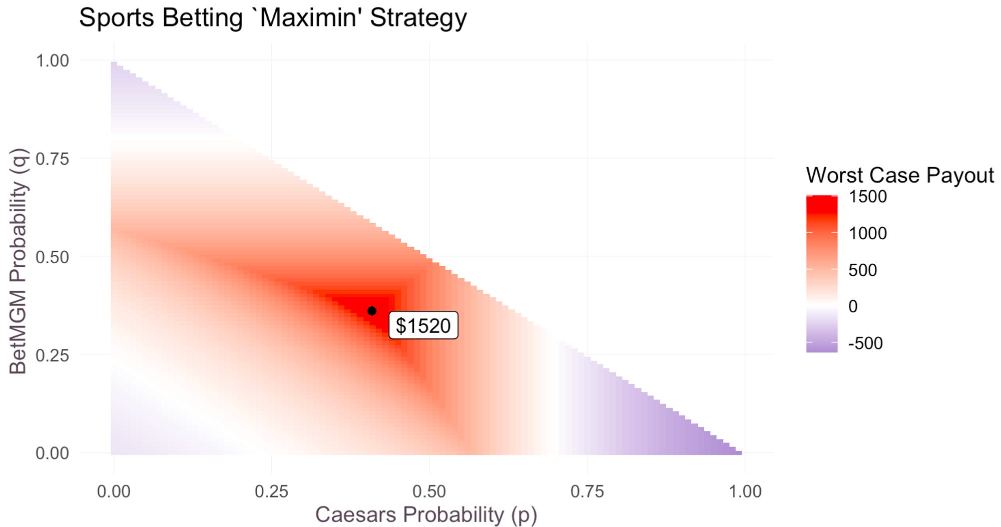
By setting p=0.41, q=0.36 (and by restriction r=0.23), one can achieve a minimum guaranteed payoff of 1520 (excluding the vig). To be clear, this is not an optimum one could luck into by placing bets arbitrarily. Much of the probability space (colored in blue) has negative worst case payoffs, and only in a narrow hill do we find guaranteed payoffs >500.
The issue with the above strategy is that when we equate payoffs across scenarios, the minimum guaranteed payoff isn’t a lower bound on EV, it is the EV. To some, this will be a desirable property in that there is no variance in payoffs whatsoever. But for those who are willing to accept some variance in payoffs to achieve higher EV, it is instructive to ask what that tradeoff looks like.
To do so, we solve the following problem:
for different values of K. This formulation asks: “what is the maximum expected value we can achieve while guaranteeing that we earn at least K dollars in the worst case scenario.” Below, we plot the values for different K:

On the far right, where we unconditionally maximize minimum guaranteed payoff, we obtain the solution above of $1520. However, as we are willing to accept lower minimum payoffs, we can raise the EV: a $1000 minimum payoff is associated with 1700 EV. With a $0 minimum payoff — a “no-loss” condition, one can raise EV to 2200. Depending on utility functions (which will pin down the optimal tradeoff), agents may choose to locate at different points on this line. The unconditional slope is -0.49, meaning for each additional dollar the agent is willing to sacrifice in guaranteed payoffs, she can obtain close to 50 cents in additional expected value.
Conclusion
That free promotions increase the EV of bets is not a particularly novel insight. It has long been acknowledged that subsidized betting offers opportunities in matched betting. The purpose of this blog post was to show how, first, how one can use portfolio optimization to convert higher EV into higher guaranteed payoffs, and second, to model certainty equivalents, i.e. how additional EV trades off with additional risk-free profit. This statistical exercise offers a number of interesting insights:
Pick your objective function (it matters!): maximizing expected values and maximizing minimum payoffs offer drastically different solutions. This difference is evident both in probability space: (p,q,r) = (0.41,0.36,0.23) vs. (p,q,r) = (0,0,1) and also in (min. payoff, EV) space: (-650,2350) vs. (1520,1520). Indeed maximizing one implicitly involves minimizing the other. This insight may seem surprising insofar as we might have thought proper portfolio optimization can achieve multiple objectives at once.
Importance of Portfolio Allocation: maximizing an objective on each individual promotion ≠ maximizing an objective across a portfolio of promotions. The key to converting EV to (risk-free) payoffs was to leverage the cross-dependence (exclusivity) of outcomes on the same event. Using promotions independently may achieve a similar EV, but sacrifices a lot of guarantees (reduced variance) relative to the aggregate portfolio optimization. This is the basic idea behind hedging and mean-variance optimization that is taught in introductory finance classes.
Side note: to further illustrate the gains from exploiting cross-dependencies, one can actually increase minimum guaranteed profit to 1565 by moving to an event with 4 exclusive outcomes, and allocating $320 to a 4th, EV=0, bet (with appropriately chosen probabilities). Even though the promotion-less fourth bet is EV=0, the dependence structure of the probabilities allows the bettor to extract higher value.
Ignore vigs at your peril: It is common to think of vigs as fixed transaction costs to be ignored. But as discussed above, they suggest that with efficient markets, promotion-less betting is a sure way to lose money over the long run. This not only implies that the EVs and payoffs above need to be adjusted downward (nonlinearly) to account for the vig, but also that the optimal probabilities themselves may change. For example, with higher vigs it becomes optimal to pick slightly lower Caesar’s probabilities and slightly higher BetMGM probabilities.
Appendix: Numeric Example
For an example of the maximin strategy at work, consider the EFL Championship soccer game featuring Blackburn vs Millwall scheduled Tuesday March 8th. Though the market-implied odds do not precisely correspond to the optimal probabilities derived above, they are relatively close and so offer a useful real-life illustration.
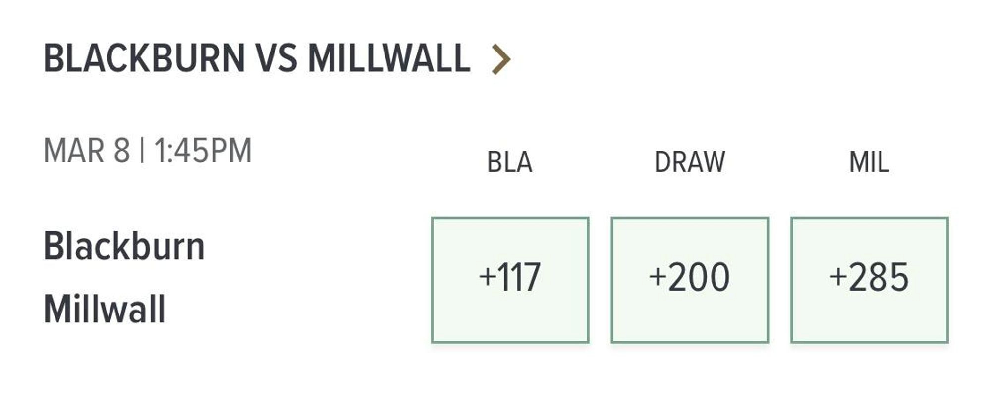
Caesars Odds: Blackburn vs. Millwall
Caesars quotes the betting odds for a Blackburn win, a draw, and a Millwall win at +117, +200, and +285 respectively. These imply outcome probabilities (”fair odds”) of 0.437, 0.316, and 0.247, with a 5.38% vig. Consider now the payoffs to a $1500 Caesars wager on a Blackburn win, a $1000 BetMGM wager on a draw, and $500 BetRivers wager on a Millwall win:
Caesars correct (Blackburn Win): Gross profit is 1755 (+117*15), less the 250 deposited at BetRivers and the 400 imputed loss on BetMGM. Net profits are thus 1105.
BetMGM correct (Draw): Gross profit is 2000 (+200*10), less the 250 deposited at BetRivers. Even though Caesars loses, its promotion fully covers the loss. Net profits are thus 1750.
BetRivers correct (Millwall Win): Gross profit is 1675 (payout of 1925 minus 250 cost of wager), less the 400 imputed loss on BetMGM. Net profits are thus 1275.
We see that regardless of what happens (and indeed, as of time of writing, this match has not happened!), the worst case profit is 1105. Due to nonzero variance (imperfect hedging) there is “upside risk” that delivers a higher expected value: